In my first personal finance post I said I had plans to write a tutorial on how to create a budget spreadsheet using Google Sheets. Well, here it is…1 year later. Josh and I just redid our budget for this year and I’m motivated again to keep using the format we have and maybe in another year I’ll share with you how we use this every month. LOL. This will be the first post of several for the tutorial. I decided to do this in parts just so it isn’t too long, they will all be linked together so finding the next part will be easy.
1. First you will want to open up a new page in Google Chrome and click on the 3×3 squares next to “image” in the top right hand corner.
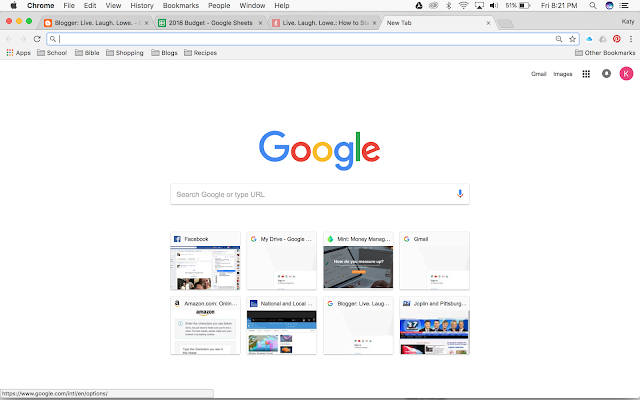
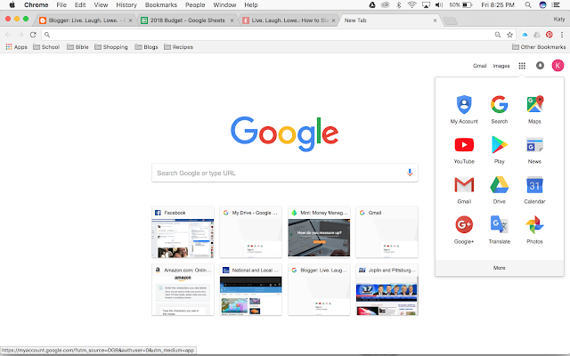
2. After clicking on the squares a drop down menu will appear and you’ll want to select “Drive”. If you don’t already have a Google account, selecting “Drive” may have you create one (it’s free so go ahead and sign up!).
3. Clicking on “Drive” will bring you to this screen. You’ll want to choose the blue button “New” and then click on “Google Sheets”.

4. Once you have opened your new Google Sheets you can name it at the top by clicking on “Untitled Spreadsheet” and typing in whatever name you want to give the document.

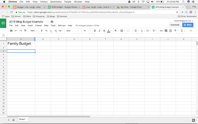
5. I also like to give the spreadsheet a title in the cell A1. But that’s just me, you don’t have to add that! My font size is 18 for those of you that want to know, and I extend the right side of the cell by clicking on the right line and dragging it.
6. Next I like to freeze columns A and B and rows 1 and 2 so that I can see them at all times. This is done by selecting row 1 and dragging down to row 2 so that both rows are light blue. Then in the ribbon below the title of your spreadsheet, select view, freeze, and 2 rows.
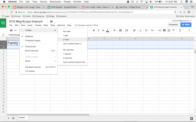
7. You’ll know that you have done it correctly when a gray line appears under row 2.
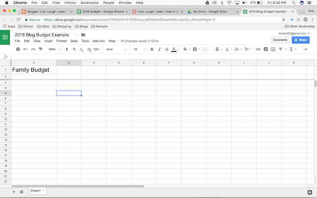
8. Repeat steps 6 on columns A and B to complete the freeze panes but instead of choosing “2 Rows” choose “2 columns”. You’ll know you have done this correctly when a gray line appears at the right edge of column B.
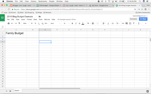
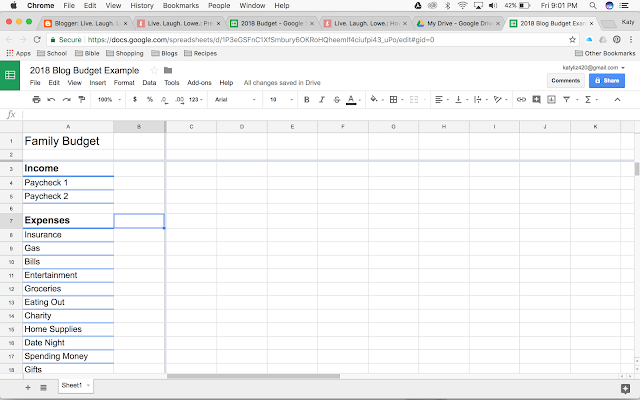
9. Next I like to add my headings for the budget categories. I’ll also write a blog soon on the different budget categories you might want to think about and the categories we use in ours. Starting in cell A3 I list out the different types of income and then in the column following I list out the different types of expenses. You can be as creative as you want with the formatting, I like to make ours easy to look at.
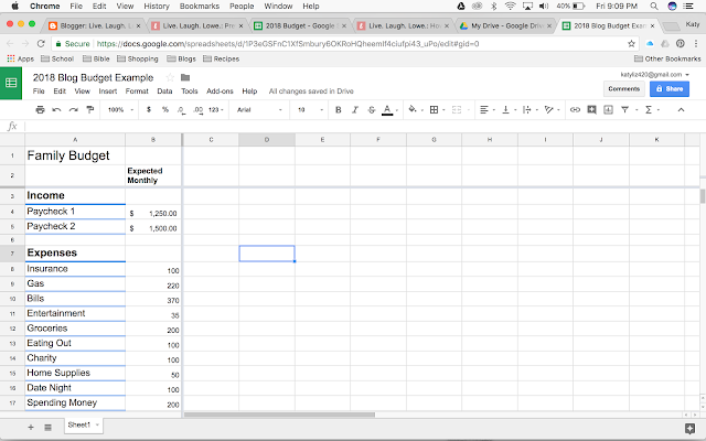
10. Next in column B you can add a header for Expected Monthly amounts and add in the dollar amounts that you’d like to see spent or earned in each month for the year. In following parts we’ll work on making sure your amounts are accurate. (I also went back later and added dollar signs to the expenses amounts).
There are the first ten steps! Stay tuned for Part 2. In total, including writing this post and capturing the screen shots while making the budget, these steps only took me 1 hour. So think how quick and easy it will be when you don’t have to write out the steps and think about how to explain the process! Let me know if you have any questions or suggestions!

